Study D — Optimal Learning Rate \(\alpha^*\) vs Problem Size \(N\)¶
Identifies the value of \(\alpha\) minimising convergence time for each \(N\), under unit sparsity (\(p_e = 1/N\)). Validates theoretical bounds from §4.3 and characterises the scaling law \(\alpha^* \propto N\) (and \(\alpha^\text{lim} \propto N\)).
Parameter |
Value |
|---|---|
Problem Size \(N\) |
[10, 1000] (20 values, log-spaced) |
Num. Parallel Nodes \(P\) |
\(\lfloor 1000 / N \rfloor\) |
Learning Rate \(\alpha\) |
[N/6, 2N/3] (50 values, log-spaced) |
Batch Size \(M\) |
50000 |
Bernouilli Prob. \(p_e\) |
\(1/N\) |
Max. Steps \(S\) |
\(\approx 30000\) |
Oracle Proportion \(p_w\) |
0.5 |
[1]:
import numpy as np
import matplotlib.pyplot as plt
import matplotlib.cm as cm
import matplotlib.colors as mcolors
import sys
import os
import glob

# Add parent directory to path
sys.path.append('..')

from plotting.plot_utility import plot_metric_vs_param, compute_steps_to_thresholds, setup_plot_style

%matplotlib inline
setup_plot_style()
[2]:
def get_latest_study_folder(study_prefix):
    pattern = f'../studies/results/{study_prefix}_*/'
    folders = glob.glob(pattern)
    if folders:
        return max(folders)  # Latest by name (timestamp-based)
    return None

mode = 'auto'  # Change to 'manual' to specify your own path

if mode == 'auto':
    results_dir = get_latest_study_folder('D_alpha_optimal')
    if results_dir is None:
        raise FileNotFoundError("No Study D results found. Run run_study_D.py first.")
    print(f"Auto-detected folder: {results_dir}")
else:
    results_dir = '../studies/results/D_alpha_optimal_XXXXXXXX_XXXXXX/'
    print(f"Using manual path: {results_dir}")

n_values = np.load(results_dir + 'n_values.npy')
optimal_alpha_per_n = np.load(results_dir + 'optimal_alpha_per_n.npy')
optimal_steps_per_n = np.load(results_dir + 'optimal_steps_per_n.npy')

print(f"\nN range: {n_values[0]} to {n_values[-1]}")
print(f"Number of N values: {len(n_values)}")
print(f"\nOptimal alpha for each N:")
for N, alpha, steps in zip(n_values, optimal_alpha_per_n, optimal_steps_per_n):
    print(f"  N={N:4d}: alpha={alpha:.6f}, steps={steps:4.0f}")

# Identify optimal and first-diverging alpha per N
alpha_value_optimal_per_N = []
alpha_value_first_divergence_per_N = []
plot_convergence = False
for N in n_values:
    alpha_values = np.load(results_dir + f'N_{N}_alpha_values.npy')
    p_diff_matrix = np.load(results_dir + f'N_{N}_p_diff_matrix.npy')

    if plot_convergence:
        plt.figure(figsize=(6, 4))

    optimal_steps = +np.inf
    alpha_id_optimal = None
    alpha_id_first_divergence = -1
    for alpha_id in range(len(alpha_values)):
        color = "blue"
        p_diff_at_alpha = p_diff_matrix[alpha_id, :]

        previous_p_diff = p_diff_at_alpha[0]
        div_threshold = 0.05
        for i in range(len(p_diff_at_alpha)):
            if np.isnan(p_diff_at_alpha[i]) or (p_diff_at_alpha[i] > div_threshold and previous_p_diff < div_threshold):
                color = 'red'
                if alpha_id_first_divergence == -1:
                    alpha_id_first_divergence = alpha_id
                break
            if p_diff_at_alpha[i] < 0.01:
                color = 'green'
                if i < optimal_steps:
                    optimal_steps = i
                    alpha_id_optimal = alpha_id
                break
            previous_p_diff = p_diff_at_alpha[i]

        if plot_convergence:
            plt.plot(p_diff_at_alpha, color=color, label=f'alpha_id={alpha_id}/alpha_value={alpha_values[alpha_id]:.6f}')

    print(f"Optimal alpha_id : {alpha_id_optimal}, alpha_value: {alpha_values[alpha_id_optimal]:.6f}")
    print(f"First alpha_id with divergence: {alpha_id_first_divergence}, alpha_value: {alpha_values[alpha_id_first_divergence]:.6f}\n")
    alpha_value_optimal_per_N.append(alpha_values[alpha_id_optimal])
    alpha_value_first_divergence_per_N.append(alpha_values[alpha_id_first_divergence])

    if plot_convergence:
        plt.yscale('log')
        plt.xlim(0, 100)
        plt.show()
Auto-detected folder: ../studies/results/D_alpha_optimal_20260420_203622/

N range: 10 to 1000
Number of N values: 20

Optimal alpha for each N:
  N=  10: alpha=3.577636, steps=   6
  N=  12: alpha=4.293163, steps=   6
  N=  16: alpha=5.724217, steps=   6
  N=  20: alpha=7.155271, steps=   6
  N=  26: alpha=9.568776, steps=   6
  N=  33: alpha=12.144985, steps=   6
  N=  42: alpha=15.026069, steps=   6
  N=  54: alpha=24.921392, steps=   5
  N=  69: alpha=31.844001, steps=   5
  N=  88: alpha=39.479739, steps=   5
  N= 112: alpha=51.688813, steps=   5
  N= 143: alpha=67.889329, steps=   5
  N= 183: alpha=84.455829, steps=   5
  N= 233: alpha=110.616878, steps=   5
  N= 297: alpha=133.244119, steps=   5
  N= 379: alpha=174.911252, steps=   5
  N= 483: alpha=222.908008, steps=   5
  N= 615: alpha=291.971589, steps=   5
  N= 784: alpha=361.821693, steps=   5
  N=1000: alpha=474.750551, steps=   5
Optimal alpha_id : 27, alpha_value: 3.577636
First alpha_id with divergence: 43, alpha_value: 5.625837

Optimal alpha_id : 27, alpha_value: 4.293163
First alpha_id with divergence: 42, alpha_value: 6.562683

Optimal alpha_id : 27, alpha_value: 5.724217
First alpha_id with divergence: 42, alpha_value: 8.750244

Optimal alpha_id : 27, alpha_value: 7.155271
First alpha_id with divergence: 42, alpha_value: 10.937805

Optimal alpha_id : 28, alpha_value: 9.568776
First alpha_id with divergence: 41, alpha_value: 13.822499

Optimal alpha_id : 28, alpha_value: 12.144985
First alpha_id with divergence: 41, alpha_value: 17.543942

Optimal alpha_id : 27, alpha_value: 15.026069
First alpha_id with divergence: 41, alpha_value: 22.328653

Optimal alpha_id : 36, alpha_value: 24.921392
First alpha_id with divergence: 41, alpha_value: 28.708268

Optimal alpha_id : 36, alpha_value: 31.844001
First alpha_id with divergence: 41, alpha_value: 36.682787

Optimal alpha_id : 35, alpha_value: 39.479739
First alpha_id with divergence: 41, alpha_value: 46.783844

Optimal alpha_id : 36, alpha_value: 51.688813
First alpha_id with divergence: 41, alpha_value: 59.543074

Optimal alpha_id : 37, alpha_value: 67.889329
First alpha_id with divergence: 41, alpha_value: 76.023747

Optimal alpha_id : 36, alpha_value: 84.455829
First alpha_id with divergence: 41, alpha_value: 97.289130

Optimal alpha_id : 37, alpha_value: 110.616878
First alpha_id with divergence: 41, alpha_value: 123.870860

Optimal alpha_id : 35, alpha_value: 133.244119
First alpha_id with divergence: 41, alpha_value: 157.895474

Optimal alpha_id : 36, alpha_value: 174.911252
First alpha_id with divergence: 41, alpha_value: 201.489511

Optimal alpha_id : 36, alpha_value: 222.908008
First alpha_id with divergence: 41, alpha_value: 256.779508

Optimal alpha_id : 37, alpha_value: 291.971589
First alpha_id with divergence: 41, alpha_value: 326.955275

Optimal alpha_id : 36, alpha_value: 361.821693
First alpha_id with divergence: 41, alpha_value: 416.801521

Optimal alpha_id : 37, alpha_value: 474.750551
First alpha_id with divergence: 41, alpha_value: 531.634593
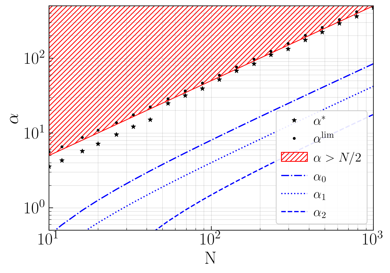
Optimal \(\alpha\) vs \(N\)¶
Empirically optimal learning rate \(\alpha^*(N)\) plotted against \(N\), alongside the theoretical bounds \(\alpha_0\), \(\alpha_1\), \(\alpha_2\) derived in §4.3. The ratio \(\alpha^*/N\) is shown to be approximately constant.
See Paper Section 5.2.3 Figure 5
[3]:
fig, ax = plt.subplots()

ax.plot(n_values, alpha_value_optimal_per_N, marker='*', color='black', linewidth=0, label='$\\alpha^*$')
ax.plot(n_values, alpha_value_first_divergence_per_N, marker='.', color='black', linewidth=0, label='$\\alpha^\\mathrm{lim}$')

a = 1/2
b = 0
ax.fill_between(n_values, a*n_values+b, 1e3, hatch="////", facecolor="none", edgecolor="red", label='$\\alpha > N/2$')

# sigma convergence bound \frac{x}{2}e^{-\frac{79x-9}{32x-72}}
bound_1 = (n_values) * np.exp(-(79 * n_values - 9) / (32 * n_values - 72))
# monotonic behaviour bound: \frac{x}{2}e^{-\frac{79x-9}{32x-72}}
bound_2 = (n_values / 2) * np.exp(-(79 * n_values - 9) / (32 * n_values - 72))
# Bounded convergence interval bound: N \times \frac{3 - 2e^{+\varepsilon(N)}}{4\times \left[\frac{3}{2} e^{9/4} e^{\eta^{(\xi)}_{\max}(N)} - e^{-1} e^{-\eta^{(\zeta)}_{\max}(N)}\right]}
epsilon = (402*n_values-216)/(2*n_values*(32*n_values-72))
eta_xi_max = 153/(32*n_values-72)
eta_zeta_max = 3/(2*n_values)
bound_3 = n_values * (3 - 2 * np.exp(+epsilon)) / (4 * (1.5 * np.exp(9 / 4) * np.exp(+eta_xi_max) - np.exp(-1) * np.exp(-eta_zeta_max)))
ax.plot(n_values, bound_1, color='blue', linestyle='-.', label='$\\alpha_0$')
ax.plot(n_values, bound_2, color='blue', linestyle=':', label='$\\alpha_1$')
ax.plot(n_values, bound_3, color='blue', linestyle='--', label='$\\alpha_2$')

ax.set_xlabel('N')
ax.set_ylabel(r'$\alpha$')
ax.set_xscale('log')
ax.set_yscale('log')
ax.set_xlim(n_values[0], n_values[-1])
ax.set_ylim(5e-1, 5e2)
ax.legend(loc='lower right')

plt.tight_layout()
plt.show()
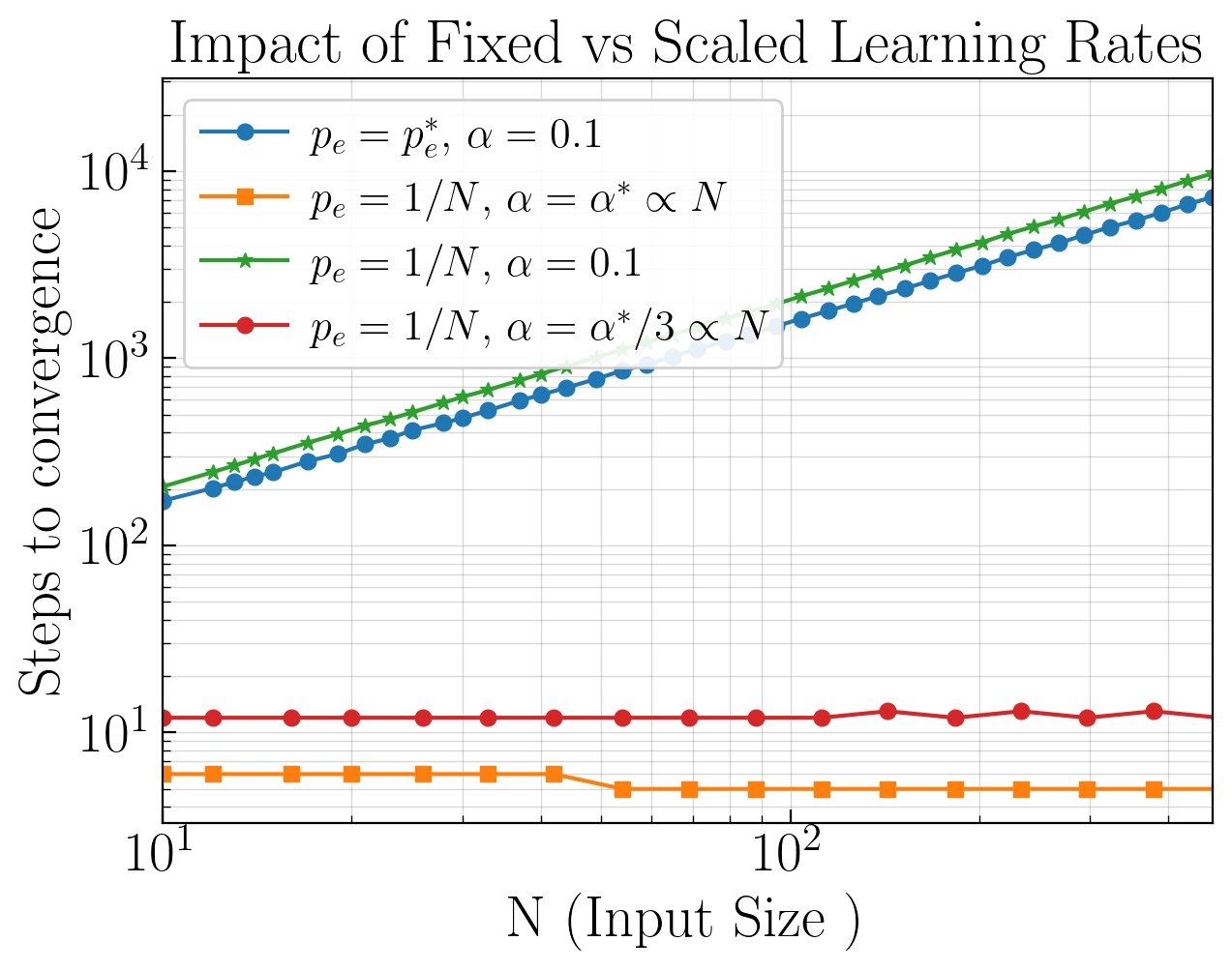
Additional Results - \(\alpha/N\) ratio¶
Relying on the results of studies B and D, shows that constant \(\alpha/N\) ratio bring constant number of steps to convergence.
[4]:
study_b_pattern = '../studies/results/B_p_e_optimal_*/'
study_b_folders = glob.glob(study_b_pattern)

if study_b_folders:
    study_b_dir = max(study_b_folders)
    print(f"Found Study B results: {study_b_dir}")

    try:
        # FROM STUDY B
        n_values_b = np.load(study_b_dir + 'n_values.npy')
        optimal_steps_b = np.load(study_b_dir + 'optimal_steps_per_n.npy')
        steps_to_convergence_at_pe_1_over_N = []

        for N in n_values_b:
            p_e_values = np.load(f"{study_b_dir}/N_{N}_p_e_values.npy")

            # Get the closest p_e index to 1/N
            target_p_e = 1 / N
            p_diff = np.abs(p_e_values - target_p_e)
            closest_index = np.argmin(p_diff)

            # Get corresponding p_diff evolution
            p_diff_matrix = np.load(f"{study_b_dir}/N_{N}_p_diff_matrix.npy")
            p_diff_at_pe_1_over_N = p_diff_matrix[closest_index, :]

            # N steps to convergence at p_e = 1/N
            found_step = False
            for step in range(len(p_diff_at_pe_1_over_N)):
                if p_diff_at_pe_1_over_N[step] < 0.01:
                    print(f"N={N}: Steps to convergence at p_e=1/N: {step}")
                    steps_to_convergence_at_pe_1_over_N.append(step)
                    found_step = True
                    break
            if not found_step:
                print(f"N={N}: Did not converge at p_e=1/N within max steps.")
                steps_to_convergence_at_pe_1_over_N.append(10000)

        # FROM STUDY D
        print(results_dir)
        n_values = np.load(results_dir + 'n_values.npy')
        optimal_steps_per_n = np.load(results_dir + 'optimal_steps_per_n.npy')
        steps_to_convergence_at_alpha_over_N = []
        for N in n_values:
            alpha_values = np.load(results_dir + f'N_{N}_alpha_values.npy')
            p_diff_matrix = np.load(results_dir + f'N_{N}_p_diff_matrix.npy')

            # Get the closest alpha index to alpha = 0.1
            target_alpha = 0.1
            alpha_diff = np.abs(alpha_values - target_alpha)
            closest_alpha_index = np.argmin(alpha_diff)
            print(f"N={N}: Closest alpha to 0.1 is {alpha_values[closest_alpha_index]:.6f} at index {closest_alpha_index}. $\alpha^*=${N/2}")

            # Get corresponding p_diff evolution
            p_diff_at_alpha = p_diff_matrix[closest_alpha_index, :]

            # N steps to convergence at alpha
            found_step = False
            for step in range(len(p_diff_at_alpha)):
                if p_diff_at_alpha[step] < 0.01:
                    print(f"N={N}: Steps to convergence at alpha: {step}")
                    steps_to_convergence_at_alpha_over_N.append(step)
                    found_step = True
                    break
            if not found_step:
                print(f"N={N}: Did not converge at alpha within max steps.")

        fig, ax = plt.subplots()
        ax.plot(n_values_b, optimal_steps_b, marker='o', label=r'$p_e=p_e^*$, $\alpha=0.1$')
        ax.plot(n_values, optimal_steps_per_n, marker='s', label=r'$p_e=1/N$, $\alpha=\alpha^* \propto N$')
        ax.plot(n_values_b, steps_to_convergence_at_pe_1_over_N, marker='*', label=r'$p_e=1/N$, $\alpha=0.1$')
        ax.plot(n_values, steps_to_convergence_at_alpha_over_N, marker='o', label=r'$p_e=1/N$, $\alpha=\alpha^*/3 \propto N$')

        ax.set_xlabel('N (Input Size )')
        ax.set_ylabel('Steps to convergence')
        ax.set_title(r"Impact of Fixed vs Scaled Learning Rates")
        ax.set_xscale('log')
        ax.set_yscale('log')
        ax.set_xlim(n_values_b[0], n_values_b[-9])

        ax.legend()

        plt.show()
    except Exception as e:
        print(f"Error loading Study B results: {e}")
else:
    print("Study B results not found. Run run_study_B.py first.")
Found Study B results: ../studies/results/B_p_e_optimal_20260420_200010/
N=10: Steps to convergence at p_e=1/N: 206
N=10: Steps to convergence at p_e=1/N: 206
N=12: Steps to convergence at p_e=1/N: 246
N=13: Steps to convergence at p_e=1/N: 267
N=14: Steps to convergence at p_e=1/N: 289
N=15: Steps to convergence at p_e=1/N: 310
N=17: Steps to convergence at p_e=1/N: 353
N=19: Steps to convergence at p_e=1/N: 393
N=21: Steps to convergence at p_e=1/N: 436
N=23: Steps to convergence at p_e=1/N: 473
N=25: Steps to convergence at p_e=1/N: 514
N=28: Steps to convergence at p_e=1/N: 578
N=30: Steps to convergence at p_e=1/N: 621
N=33: Steps to convergence at p_e=1/N: 677
N=37: Steps to convergence at p_e=1/N: 761
N=40: Steps to convergence at p_e=1/N: 823
N=44: Steps to convergence at p_e=1/N: 907
N=49: Steps to convergence at p_e=1/N: 1006
N=54: Steps to convergence at p_e=1/N: 1114
N=59: Steps to convergence at p_e=1/N: 1214
N=65: Steps to convergence at p_e=1/N: 1341
N=71: Steps to convergence at p_e=1/N: 1462
N=79: Steps to convergence at p_e=1/N: 1629
N=86: Steps to convergence at p_e=1/N: 1768
N=95: Steps to convergence at p_e=1/N: 1950
N=104: Steps to convergence at p_e=1/N: 2142
N=115: Steps to convergence at p_e=1/N: 2362
N=126: Steps to convergence at p_e=1/N: 2599
N=138: Steps to convergence at p_e=1/N: 2849
N=152: Steps to convergence at p_e=1/N: 3126
N=167: Steps to convergence at p_e=1/N: 3451
N=184: Steps to convergence at p_e=1/N: 3804
N=202: Steps to convergence at p_e=1/N: 4162
N=222: Steps to convergence at p_e=1/N: 4606
N=244: Steps to convergence at p_e=1/N: 5054
N=268: Steps to convergence at p_e=1/N: 5512
N=294: Steps to convergence at p_e=1/N: 6074
N=323: Steps to convergence at p_e=1/N: 6694
N=355: Steps to convergence at p_e=1/N: 7319
N=390: Steps to convergence at p_e=1/N: 8014
N=429: Steps to convergence at p_e=1/N: 8872
N=471: Steps to convergence at p_e=1/N: 9698
N=517: Steps to convergence at p_e=1/N: 10674
N=568: Steps to convergence at p_e=1/N: 11692
N=625: Steps to convergence at p_e=1/N: 12872
N=686: Steps to convergence at p_e=1/N: 14084
N=754: Steps to convergence at p_e=1/N: 15448
N=828: Steps to convergence at p_e=1/N: 17096
N=910: Steps to convergence at p_e=1/N: 18840
N=1000: Steps to convergence at p_e=1/N: 20686
../studies/results/D_alpha_optimal_20260420_203622/
N=10: Closest alpha to 0.1 is 1.666667 at index 0. $lpha^*=$5.0
N=10: Steps to convergence at alpha: 12
N=12: Closest alpha to 0.1 is 2.000000 at index 0. $lpha^*=$6.0
N=12: Steps to convergence at alpha: 12
N=16: Closest alpha to 0.1 is 2.666667 at index 0. $lpha^*=$8.0
N=16: Steps to convergence at alpha: 12
N=20: Closest alpha to 0.1 is 3.333333 at index 0. $lpha^*=$10.0
N=20: Steps to convergence at alpha: 12
N=26: Closest alpha to 0.1 is 4.333333 at index 0. $lpha^*=$13.0
N=26: Steps to convergence at alpha: 12
N=33: Closest alpha to 0.1 is 5.500000 at index 0. $lpha^*=$16.5
N=33: Steps to convergence at alpha: 12
N=42: Closest alpha to 0.1 is 7.000000 at index 0. $lpha^*=$21.0
N=42: Steps to convergence at alpha: 12
N=54: Closest alpha to 0.1 is 9.000000 at index 0. $lpha^*=$27.0
N=54: Steps to convergence at alpha: 12
N=69: Closest alpha to 0.1 is 11.500000 at index 0. $lpha^*=$34.5
N=69: Steps to convergence at alpha: 12
N=88: Closest alpha to 0.1 is 14.666667 at index 0. $lpha^*=$44.0
N=88: Steps to convergence at alpha: 12
N=112: Closest alpha to 0.1 is 18.666667 at index 0. $lpha^*=$56.0
N=112: Steps to convergence at alpha: 12
N=143: Closest alpha to 0.1 is 23.833333 at index 0. $lpha^*=$71.5
N=143: Steps to convergence at alpha: 13
N=183: Closest alpha to 0.1 is 30.500000 at index 0. $lpha^*=$91.5
N=183: Steps to convergence at alpha: 12
N=233: Closest alpha to 0.1 is 38.833333 at index 0. $lpha^*=$116.5
N=233: Steps to convergence at alpha: 13
N=297: Closest alpha to 0.1 is 49.500000 at index 0. $lpha^*=$148.5
N=297: Steps to convergence at alpha: 12
N=379: Closest alpha to 0.1 is 63.166667 at index 0. $lpha^*=$189.5
N=379: Steps to convergence at alpha: 13
N=483: Closest alpha to 0.1 is 80.500000 at index 0. $lpha^*=$241.5
N=483: Steps to convergence at alpha: 12
N=615: Closest alpha to 0.1 is 102.500000 at index 0. $lpha^*=$307.5
N=615: Steps to convergence at alpha: 13
N=784: Closest alpha to 0.1 is 130.666667 at index 0. $lpha^*=$392.0
N=784: Steps to convergence at alpha: 13
N=1000: Closest alpha to 0.1 is 166.666667 at index 0. $lpha^*=$500.0
N=1000: Steps to convergence at alpha: 13
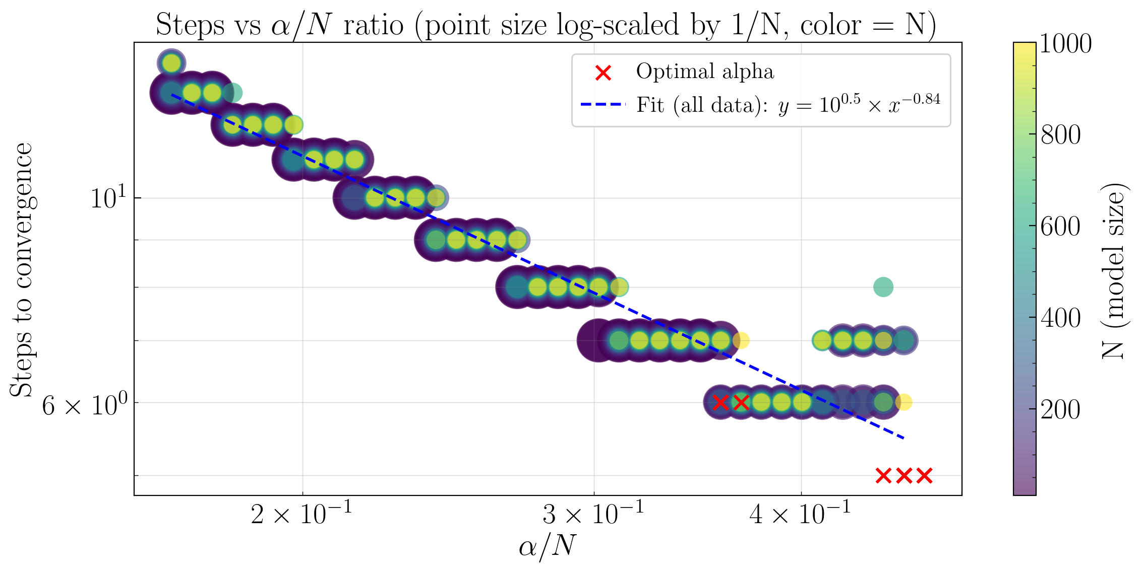
[5]:
# Same for all alpha values below optimal (not only optimal alpha)
n_values = np.load(results_dir + 'n_values.npy')
optimal_alpha_per_n = np.load(results_dir + 'optimal_alpha_per_n.npy')
optimal_steps_per_n = np.load(results_dir + 'optimal_steps_per_n.npy')

print(f"\nN range: {n_values[0]} to {n_values[-1]}")

fig, ax = plt.subplots(figsize=(12, 6))

# Create a colormap
import matplotlib.cm as cm
from matplotlib.colors import Normalize

# Normalize N values for color mapping
norm = Normalize(vmin=n_values.min(), vmax=n_values.max())
cmap = cm.viridis

# Collect all points for scatter plot with color and size based on N
all_ratios = []
all_steps = []
all_n_values = []

for N, optimal_alpha in zip(n_values, optimal_alpha_per_n):
    alpha_per_n = np.load(results_dir + f'N_{N}_alpha_values.npy')
    steps_per_n = np.load(results_dir + f'N_{N}_steps.npy')
    for alpha, steps in zip(alpha_per_n, steps_per_n):
        if alpha < optimal_alpha:
            print(f"  N={N:4d}: alpha={alpha:.6f}, steps={steps:4.0f}", end='\r')
            alpha_over_n_ratio = alpha / N
            all_ratios.append(alpha_over_n_ratio)
            all_steps.append(steps)
            all_n_values.append(N)

# Convert to arrays
all_ratios = np.array(all_ratios)
all_steps = np.array(all_steps)
all_n_values = np.array(all_n_values)

# Size with logarithmic scale: smaller N = larger points (for background visibility)
sizes = 500 * np.log10(n_values.max() / all_n_values + 1)

# Create scatter plot with colorbar and variable sizes
scatter = ax.scatter(all_ratios, all_steps, c=all_n_values, cmap=cmap,
                     norm=norm, s=sizes, alpha=0.6, edgecolors='none')

# Add optimal points as red crosses on top
optimal_ratios = optimal_alpha_per_n / n_values
ax.scatter(optimal_ratios, optimal_steps_per_n, c='red', marker='x', s=100,
           linewidths=2, label='Optimal alpha', zorder=10)

# Fit a line through all data points in log-log space
log_all_ratios = np.log10(all_ratios)
log_all_steps = np.log10(all_steps)
coeffs = np.polyfit(log_all_ratios, log_all_steps, 1)
fit_ratios = np.logspace(np.log10(all_ratios.min()), np.log10(all_ratios.max()), 100)
fit_steps = 10**(coeffs[0] * np.log10(fit_ratios) + coeffs[1])
ax.plot(fit_ratios, fit_steps, 'b--', linewidth=2,
        label=f'Fit (all data): $y = 10^{{{coeffs[1]:.1f}}} \\times x^{{{coeffs[0]:.2f}}}$', zorder=9)

# Add colorbar
cbar = plt.colorbar(scatter, ax=ax, label='N (model size)')

ax.set_xscale('log')
ax.set_yscale('log')
ax.set_xlabel('$\\alpha / N$')
ax.set_ylabel('Steps to convergence')
ax.set_title('Steps vs $\\alpha/N$ ratio (point size log-scaled by 1/N, color = N)')
ax.legend()
ax.grid(True, alpha=0.3)
plt.tight_layout()
plt.show()
N range: 10 to 1000
  N=1000: alpha=461.507262, steps=   6