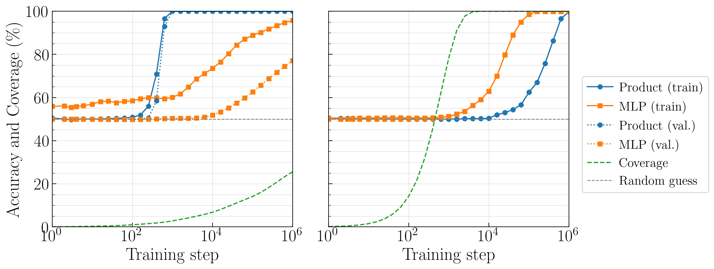
Study H — Product Node vs MLP: Sparse vs Full-Table Training
Compares a product node with a standard MLP under two training regimes:
Sparse: Bernouilli sampled inputs with \(p_e = 1/N\) (very few active bits per example).
Full: inputs sampled uniformly from the complete truth table (\(2^N\) rows).
Both models are evaluated on the full truth table (generalisation accuracy).
Parameter |
Value |
|---|---|
Problem Size \(N\) |
16 |
Truth Table Size \(2^N\) |
65 536 |
Num. Parallel Nodes. \(P\) |
250 |
Learning Rate \(\alpha\) |
0.02 |
Batch Size \(M\) |
100 |
Bernouilli Prob. \(p_e\) |
\(1/N\) or uniform TT sampling |
Oracle Proportion \(p_w\) |
0.5 |
Max. Steps \(S\) |
1 000 000 |
MLP Architecture |
\(N \to 512 \to 512 \to 64 \to 1\) |
[1]:
import numpy as np
import matplotlib.pyplot as plt
import sys
import os
import glob

sys.path.append('..')
from plotting.plot_utility import setup_plot_style

%matplotlib inline
setup_plot_style()
[2]:
def get_latest_study_folder(study_prefix):
    pattern = f'../studies/results/{study_prefix}_*/'
    folders = glob.glob(pattern)
    if folders:
        return max(folders)  # Latest by name (timestamp-based)
    return None

mode = 'auto'  # Change to 'manual' to specify your own path

if mode == 'auto':
    results_dir = get_latest_study_folder('H_product_vs_mlp')
    if results_dir is None:
        raise FileNotFoundError("No Study H results found. Run run_study_H.py first.")
    print(f"Auto-detected folder: {results_dir}")
else:
    results_dir = '../studies/results/H_product_vs_mlp_XXXXXX_XXXXXX/'
    print(f"Using manual path: {results_dir}")

# ---- Load arrays ----
# Training accuracy on seen codewords
sparse_product_train_acc = np.load(results_dir + 'sparse_product_train_acc.npy')
sparse_mlp_train_acc     = np.load(results_dir + 'sparse_mlp_train_acc.npy')
full_product_train_acc   = np.load(results_dir + 'full_product_train_acc.npy')
full_mlp_train_acc       = np.load(results_dir + 'full_mlp_train_acc.npy')

# Validation accuracy on full truth table
sparse_product_val_acc = np.load(results_dir + 'sparse_product_val_acc.npy')
sparse_mlp_val_acc     = np.load(results_dir + 'sparse_mlp_val_acc.npy')
full_product_val_acc   = np.load(results_dir + 'full_product_val_acc.npy')
full_mlp_val_acc       = np.load(results_dir + 'full_mlp_val_acc.npy')

# Coverage and eval steps
sparse_coverage = np.load(results_dir + 'sparse_coverage.npy')
full_coverage   = np.load(results_dir + 'full_coverage.npy')
eval_steps      = np.load(results_dir + 'eval_steps.npy')

n_runs = sparse_product_train_acc.shape[0]

print(f"Loaded: {n_runs} runs, {len(eval_steps)} eval points")
print(f"Eval steps range: {eval_steps[0]:.0f} to {eval_steps[-1]:.0f}")
print(f"Sparse coverage (final): {100*sparse_coverage[:,-1].mean():.4f}%")
print(f"Full   coverage (final): {100*full_coverage[:,-1].mean():.2f}%")
Auto-detected folder: ../studies/results/H_product_vs_mlp_20260420_233719/
Loaded: 1 runs, 31 eval points
Eval steps range: 1 to 1000000
Sparse coverage (final): 25.5936%
Full   coverage (final): 100.00%
Generalisation Accuracy — Sparse vs Full Training Regime
Left (Sparse): The product node generalises perfectly from very few examples (\(\ll 1\%\) coverage), while the MLP overfits to the training set (discrepancies between training and validation accuracies).
Right (Full): With uniform sampling, both models eventually learn. The MLP is faster than the product node but requires complete coverage.
Solid lines = training accuracy (seen codewords). Dashed lines = validation accuracy (full truth table). Green dotted = coverage (\(\%\) of \(2^N\) unique inputs seen).
See Paper Section 5.2.4. Figure 6.
[3]:
fig, (ax_sp, ax_fu) = plt.subplots(
    1,
    2,
    figsize=(
        plt.rcParams['figure.figsize'][0] * 1.5,
        plt.rcParams['figure.figsize'][1] * 1
    ),
    sharey=True)

color_prod = 'tab:blue'
color_mlp  = 'tab:orange'
color_cov  = 'tab:green'

for ax, regime, prod_tr, mlp_tr, prod_val, mlp_val, cov, title in [
    (ax_sp, 'sparse',
     sparse_product_train_acc, sparse_mlp_train_acc,
     sparse_product_val_acc,   sparse_mlp_val_acc,
     sparse_coverage,          r'Sparse Regime ($p_e = 1/N$)'),
    (ax_fu, 'full',
     full_product_train_acc,   full_mlp_train_acc,
     full_product_val_acc,     full_mlp_val_acc,
     full_coverage,            r'Dense Regime (uniform)'),
]:
    # Mean and std across runs
    pt_m, pt_s = prod_tr.mean(0),  prod_tr.std(0)
    mt_m, mt_s = mlp_tr.mean(0),   mlp_tr.std(0)
    pv_m, pv_s = prod_val.mean(0), prod_val.std(0)
    mv_m, mv_s = mlp_val.mean(0),  mlp_val.std(0)

    # Training accuracy (solid)
    ax.plot(eval_steps, pt_m, color=color_prod, ls='-', marker='o', label='Product (train)')
    #ax.fill_between(eval_steps, pt_m - pt_s, pt_m + pt_s, color=color_prod, alpha=0.12)
    ax.plot(eval_steps, mt_m, color=color_mlp, ls='-', marker='s', label='MLP (train)')
    #ax.fill_between(eval_steps, mt_m - mt_s, mt_m + mt_s, color=color_mlp, alpha=0.12)

    # Validation accuracy (dashed)
    ax.plot(eval_steps, pv_m, color=color_prod, ls=':', marker='o', label='Product (val.)')
    #ax.fill_between(eval_steps, pv_m - pv_s, pv_m + pv_s, color=color_prod, alpha=0.08)
    ax.plot(eval_steps, mv_m, color=color_mlp, ls=':', marker='s', label='MLP (val.)')
    #ax.fill_between(eval_steps, mv_m - mv_s, mv_m + mv_s, color=color_mlp, alpha=0.08)

    # Coverage (dotted, same axis)
    cov_m = 100 * cov.mean(0)
    cov_s = 100 * cov.std(0)
    ax.plot(eval_steps, cov_m, color=color_cov, ls='--', label='Coverage')
    #ax.fill_between(eval_steps, cov_m - cov_s, cov_m + cov_s, color=color_cov, alpha=0.10)

    # Random guess baseline
    ax.axhline(50, color='grey', ls='--', lw=1.0, label='Random guess')

    ax.set_xlabel('Training step')
    ax.set_xscale('log')
    ax.set_xlim(1, eval_steps[-1])
    ax.set_ylim(0, 100)
    #ax.set_title(title)

# Left plot gets the y-label
ax_sp.set_ylabel('Accuracy and Coverage (\\%)')

# Single shared legend outside both plots
handles, labels = ax_sp.get_legend_handles_labels()
fig.legend(handles, labels, loc='center right', bbox_to_anchor=(1.2, 0.5))

plt.tight_layout()
plt.show()